vLLM: LLM Inference as a memory and scheduling problem

16 min read

Running an LLM is easy.

outputs=model.generate(...)

There. Inference solved.

This works surprisingly well when there is one model, one prompt, one GPU, and nobody asking why the first token took six seconds. There is no request queue. No streaming client that disconnects halfway through. No 32K context eating several gigabytes of memory. No product manager wondering why doubling traffic caused p99 latency to quadruple.

Under those conditions, almost anything looks like an inference engine.

Serving an LLM is a different problem. The model still performs the same transformer operations, but the system around it now has to answer a less glamorous set of questions:

Which requests should run next?
How many tokens should be processed in one step?
Where should their key-value caches live?
What happens when the GPU runs out of cache space?
How do we mix a new 20,000-token prompt with fifty users who are already waiting for their next token?

This is where vLLM comes in.

Over the last year, I’ve used vLLM at both ends of the scale, from benchmarking small models on a consumer GPU to deploying large, long-context models across multiple nodes. The hardware, workload, and failure modes were very different, but the same lessons kept showing up.

vLLM is not primarily a faster implementation of a transformer forward pass.It is a system for deciding which forward pass should happen next, which tokens should be packed into it, and where the state required by those tokens should be stored.

The two central problems are memory management and scheduling.

The attention kernels still matter. So do quantization, CUDA graphs, distributed collectives, and all the other things that make GPU engineers stare at traces until their eyes stop focusing. But none of those help much if the engine wastes half its memory or feeds the GPU the wrong work.

What sits between the request and GPU?

For online serving, a vLLM request moves through three main parts of the system:

The API server deals with the outside world. It accepts requests, performs input processing, and streams generated tokens back to the client.
The Engine Core owns the serving state. It runs the scheduler, manages the KV cache, and coordinates model execution.
The GPU workers hold the model weights and execute the forward passes. In distributed deployments, there may be several workers, with one worker process managing each GPU.

The full architecture becomes more complicated once data parallelism and multi-node execution enter the picture, but this simplified view is enough for now.

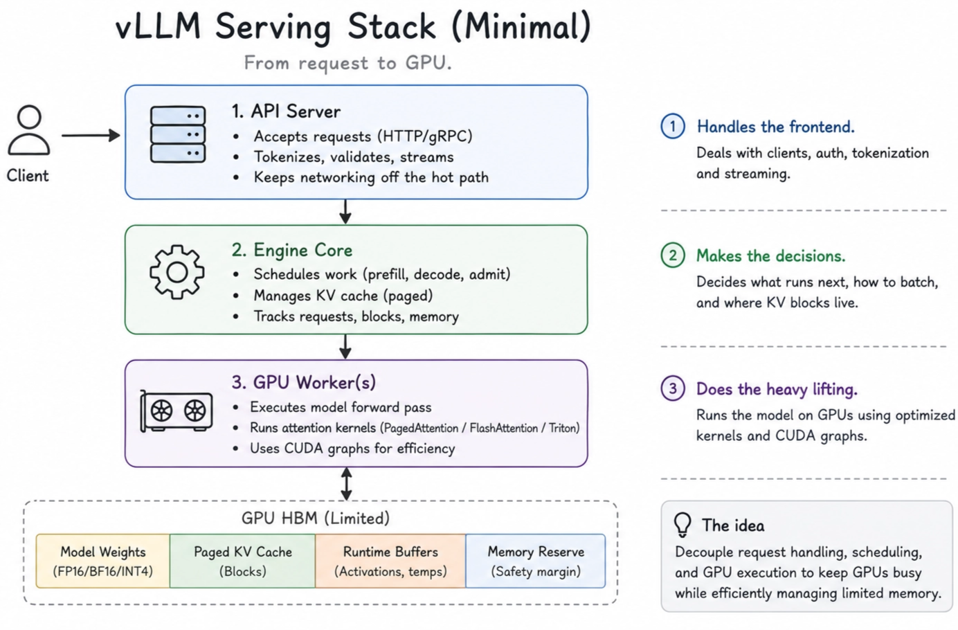
vLLM separates request handling, scheduling, and GPU execution. The Engine Core decides which token work runs and where its KV state lives.

The interesting part is the Engine Core. A normal application might send a tensor to the GPU and wait for the result. An inference server has a changing collection of requests, each at a different stage, with a different sequence length and a different amount of memory already allocated.

Before looking at how vLLM manages them together, we first need to separate the two types of work inside a single request.

One request, two workloads

An autoregressive LLM request has two phases: prefill and decode.

They pass through the same model, but they behave very differently on the hardware.

Prefill: the model reads

During prefill, the model processes the input prompt. If the user sends 2,000 tokens, the model can process those tokens together through relatively large matrix multiplications.This is where the model builds the key-value cache for the prompt and produces the first output token.

Prefill therefore contributes heavily to time-to-first-token, usually shortened to TTFT.

Large prompts tend to have enough parallel work to use the GPU's compute units efficiently, so prefill is often compute-bound. That is a useful approximation, not a law. Small prompts, small models, awkward tensor shapes, and framework overhead can move the bottleneck elsewhere.

Decode: the model types

After the first token, generation becomes autoregressive.

The model generates one new token for each active sequence, appends its key and value to the cache, and repeats.

One token. Another forward pass. One token. Another forward pass.

The operations are much smaller than prefill, but each step has to read the model weights and attend over the existing KV history. As the context grows, more KV data must be read for every new token.

Decode is therefore often limited by memory bandwidth, launch overhead, or both. Its user-facing metric is inter-token latency, or ITL.

A useful approximation is:

Prefill is the model reading the prompt. Decode is the model typing the answer.

A single request contains two hardware workloads. Prefill processes the prompt in parallel. Decode produces one token at a time while repeatedly reading the growing KV cache.

The problem is that an inference server has to handle both workloads at once.

A new request may arrive with a long prompt while dozens of existing requests are decoding. Processing the entire prompt immediately gives the new request a good TTFT, but everyone already decoding has to wait. Prioritizing decode protects ITL, but the new request may sit in the queue long enough for the user to assume the server has died.

The scheduler has to balance these workloads on the same GPU. Continuous batching, chunked prefill, token budgets, and admission control all exist because prefill and decode want different things.

This distinction also explains why “GPU utilization” is a fairly unhelpful answer by itself. A GPU can show low utilization because the decode batch is too small. It can show high utilization while tail latency is terrible because long prefills are blocking active decodes. It can be full of KV cache while its compute units remain underused.

The percentage is a symptom. It is not the diagnosis .Before the scheduler can decide which requests should run, the memory manager has to make enough room to keep them resident.

That brings us to the KV cache.

The KV cache ate my GPU

During autoregressive generation, every attention layer needs access to the keys and values produced by earlier tokens.

Recomputing them from scratch during every decode step would be absurdly expensive, so inference engines retain them in the KV cache.

For a conventional decoder-only transformer, the approximate KV-cache memory required per token is:

M_{t o k e n} = 2 \times L \times H_{K V} \times d_{head} \times B

where:

$L$ is the number of transformer layers
$H_{K V}$ is the number of key-value heads
$d_{h e a d}$ is the head dimension
$B$ is the number of bytes per element
the factor of two accounts for both keys and values

Take Qwen3-1.7B as a small example. Its configuration has:

28 transformer layers
8 KV heads
a head dimension of 128

With an FP16 KV cache, each element takes two bytes:

M_{t o k e n} = 2 \times 28 \times 8 \times 128 \times 2 = 114, 688 bytes

That is 112 KiB per token. One full 32K sequence therefore needs roughly 3.5 GiB of KV cache.

The raw 16-bit weight footprint of a 1.7B-parameter model is around 3.2 GiB. One long request can occupy roughly as much KV memory as the entire model.

And this is a small model using grouped-query attention. Larger models, longer contexts, more concurrent sequences, or more KV heads make the problem worse.

Qwen3-1.7B is a small model, but one full 32K FP16 KV cache is roughly the same size as its weights. Add concurrency and KV quickly becomes the dominant memory consumer.

Total KV use scales with the number of resident tokens across every active sequence:

M_{KV,total} \approx M_{token} \times \sum_{i} sequence length_{i}

This is why “the model fits on the GPU” is not enough information.

A large model may fit after tensor parallelism or quantization while leaving little room for requests. A small model may fit comfortably and still run out of memory once enough long sequences are resident. A deployment configured for a theoretical 128K context may support very little useful concurrency, even if most requests are much shorter.

Weights are mostly static. KV memory grows and shrinks as requests arrive, generate tokens, finish, get preempted, or reuse cached prefixes.

LLM serving is a dynamic memory-allocation problem wearing a transformer costume.

Why the obvious allocation strategy is bad

The simplest KV-cache design is to reserve a contiguous buffer for every request.

If the maximum context length is 32K, allocate enough space for 32K tokens as soon as the request begins.

Simple. Predictable. Also extremely wasteful.

Most requests will not consume their full allocation. One may stop after 200 tokens. Another after 4,000. Another may continue for 20,000 because the model decided the user needed a small autobiography before receiving the answer. The output length is not even known in advance. It depends on the model, sampling settings, stop conditions, and what the user asked for.

This produces two familiar allocator problems:

Internal fragmentation happens when a request receives more memory than it uses.

External fragmentation happens when enough free memory exists in total, but it is split into pieces that cannot satisfy a large contiguous allocation.

Contiguous allocation reserves memory around a request’s possible future length. Paged allocation reserves only the blocks that currently exist.

For an LLM server, wasted KV memory means fewer active sequences. Fewer active sequences mean smaller decode batches. Smaller decode batches mean the GPU spends more time reading weights to produce fewer tokens.

A memory problem becomes a throughput problem. This observation is central to the original PagedAttention work. By reducing fragmentation and redundant KV duplication, vLLM was able to sustain larger batches. The paper reported two to four times higher throughput than FasterTransformer and Orca at a similar level of latency.

This is the problem PagedAttention was designed to solve.

PagedAttention: virtual memory, but for tokens

PagedAttention borrows its central idea from operating systems.

A process sees a contiguous virtual address space. The physical pages backing that space can be scattered across RAM. The operating system uses a page table to translate from virtual pages to physical frames.

vLLM applies a similar abstraction to the KV cache.

Each sequence has an ordered series of logical KV blocks. The corresponding physical blocks can live anywhere in the GPU’s KV-cache pool. A block table maps each logical block to its physical location.

Suppose a sequence contains 64 tokens and the block size is 16 tokens. It needs four logical blocks:

Logical block 0: tokens  0–15
Logical block 1: tokens 16–31
Logical block 2: tokens 32–47
Logical block 3: tokens 48–63

Those blocks do not need to sit next to each other in GPU memory:

Logical block 0 → Physical block 4
Logical block 1 → Physical block 9
Logical block 2 → Physical block 2
Logical block 3 → Physical block 6

From the request’s point of view, its KV history is ordered and continuous. Physically, the allocator uses whichever blocks are free.

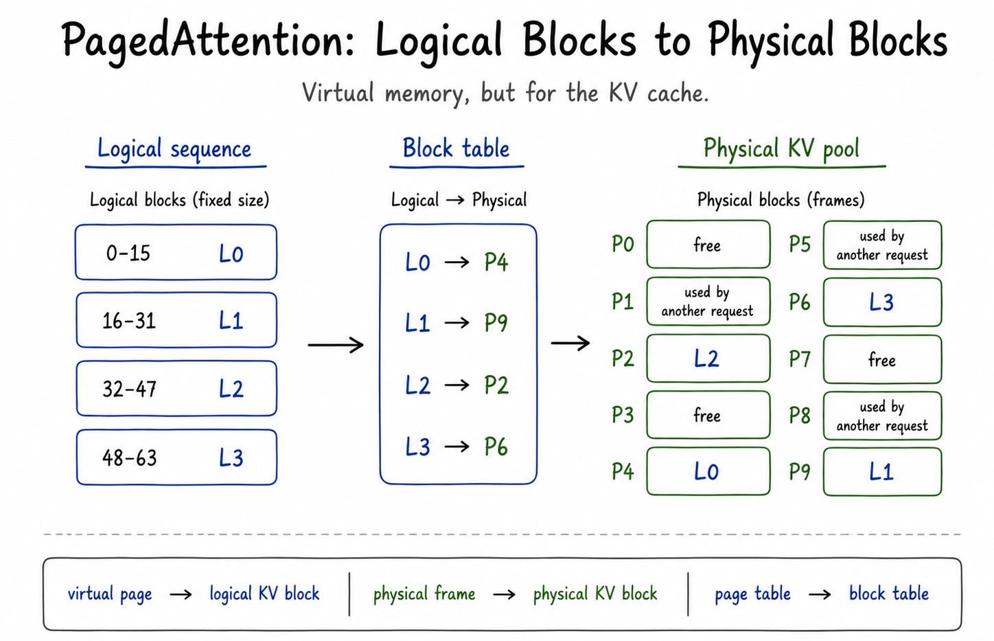
A sequence sees an ordered logical KV history even though its physical blocks are scattered across GPU memory. The block table performs the translation.

When a sequence grows, vLLM allocates another physical block. When it finishes, its blocks return to the pool. There is no need to reserve enough memory for the maximum possible context length in advance.

External fragmentation is largely avoided because allocations use the same fixed-size unit. Internal waste is mostly limited to unused positions in the final partially filled block.

A smaller block size reduces that final-block waste but increases metadata and bookkeeping. A larger block size reduces metadata but can leave more unused space. As usual, the right trade-off depends on the workload and backend.

Watching a sequence grow

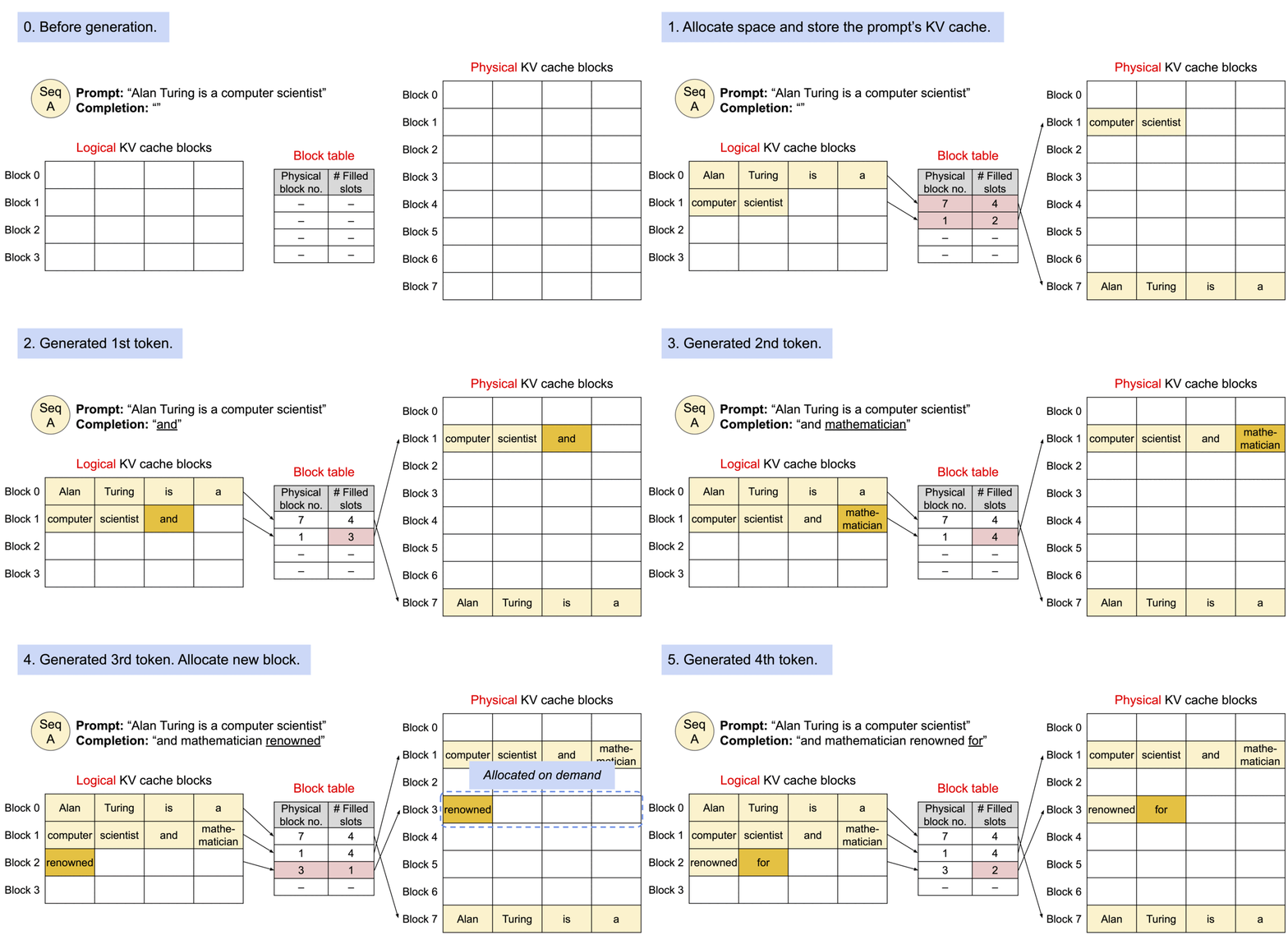
A static block-table diagram explains the mapping, but it does not show the most useful part of paging: sequences can grow incrementally.

A request begins with enough blocks to hold its prompt. Decode tokens fill the final partial block one at a time. Only when that block becomes full does the allocator request another physical block, which can come from anywhere in the free pool.

KV blocks are allocated as the sequence grows rather than reserved for the maximum possible output length.

The block abstraction also enables sharing.

The original PagedAttention design used reference-counted blocks and copy-on-write so requests with a shared prefix did not always need duplicate physical storage. Modern automatic prefix caching uses the same block granularity to reuse completed KV blocks when a later request has a matching prefix.

There is an important qualifier: only completed blocks are reusable. The final partial block is still being appended to, so it cannot be treated as an immutable cached prefix.

Prefix caching deserves its own discussion in Part 2. For now, the important point is that paging lets allocation follow a request's actual growth rather than its theoretical maximum.

Paging is not free

PagedAttention introduces indirection.

With an ordinary contiguous tensor, the attention kernel already knows where the next part of the KV history lives. With paging, it needs metadata describing how logical blocks map to physical storage.

The block table has to be maintained and consumed by the attention backend. A sequence's history may span several physical blocks.

There is a cost. The useful question is not whether the cost exists. It is whether that cost is smaller than the cost of wasting enough memory to reduce serving concurrency. For dynamic workloads, it usually is.

A block is still a regular contiguous region. The kernel is not chasing an arbitrary pointer for every scalar value. It follows a compact mapping and processes contiguous data within each block.The system trades a manageable amount of metadata and indirection for much better global memory utilization.

PagedAttention does not make one isolated attention operation magically cheaper. It lets the serving system keep more useful work resident, which can create larger decode batches and better GPU efficiency.

FlashAttention is not PagedAttention

PagedAttention and FlashAttention are frequently mixed together because both involve attention and GPU memory.

They solve different problems.

FlashAttention changes how attention is computed

A naïve attention implementation may materialize large intermediate tensors and repeatedly move data between high-bandwidth GPU memory and the much smaller, faster on-chip memory.

FlashAttention tiles the operation to reduce those reads and writes. It computes exact attention without materializing the full attention matrix in HBM.

Its question is:

How do we calculate attention without moving more data than necessary?

PagedAttention changes how persistent KV is stored

PagedAttention organizes the long-lived KV cache into blocks and maps each sequence's logical history to physical GPU memory.

Its question is:

Where does the KV cache live, and how can many dynamic sequences share memory efficiently?

A compact distinction is:

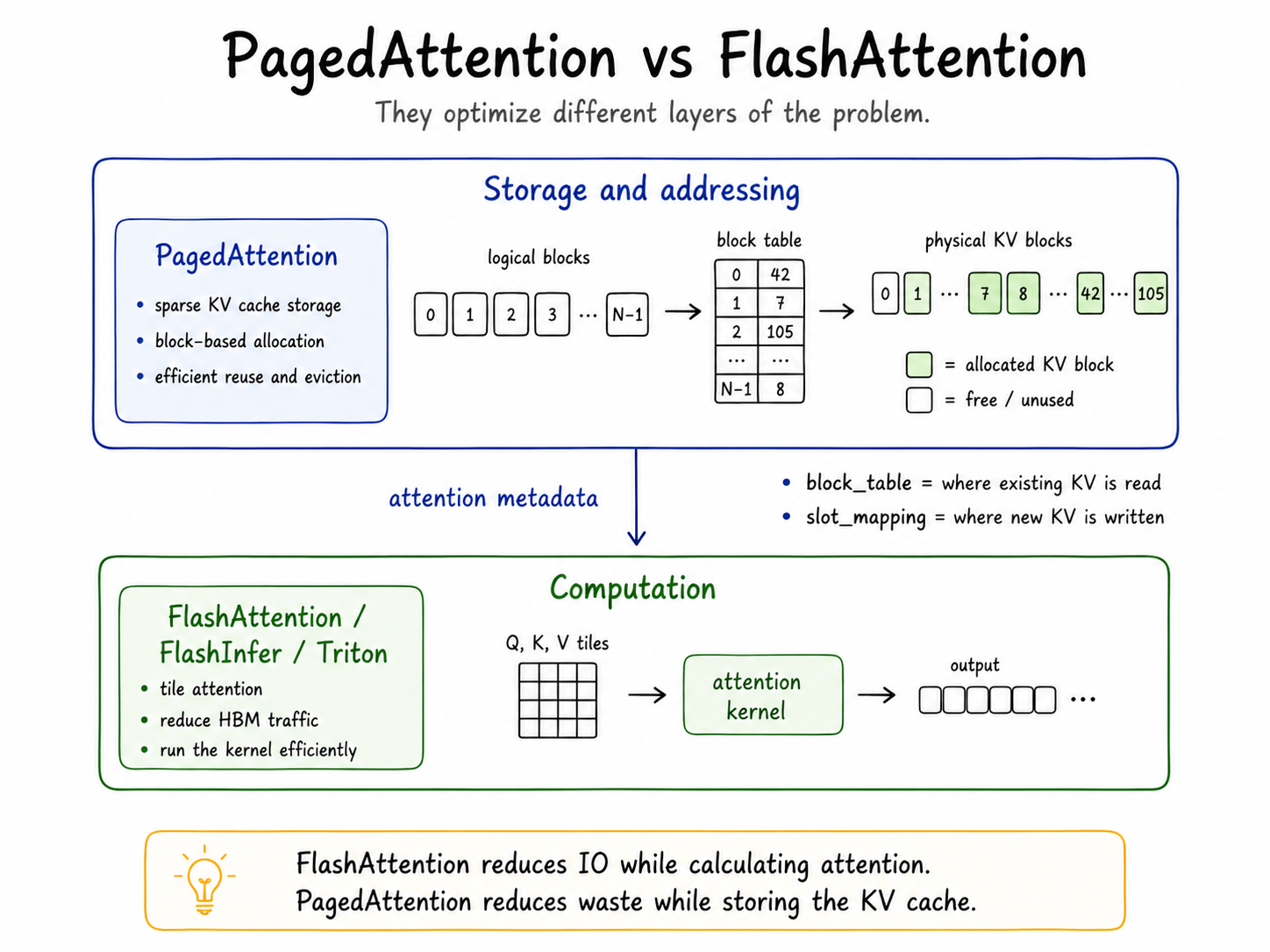
FlashAttention reduces IO while computing attention. PagedAttention reduces waste while storing the KV cache.

They are complementary.

vLLM can store KV in paged blocks while an optimized attention backend performs the actual attention operation.

PagedAttention determines where persistent KV lives. The attention backend determines how the operation is executed. The two techniques optimize different layers of the serving stack.

How an attention backend consumes paged KV

Before a model step runs, the scheduler and KV-cache manager prepare metadata describing the selected batch.

The exact representation varies by backend and vLLM version, but it needs to communicate information such as:

where each sequence's existing KV blocks live
where newly computed keys and values should be written
the current sequence lengths and query positions
the boundaries of the ragged batch

Two useful pieces of metadata are the block table and slot mapping.

The block table tells the backend where the existing KV history is stored. The slot mapping tells it where newly computed keys and values should be written.

A useful shorthand is:

The block table reads history. The slot mapping appends state.

The attention backend then operates on the paged representation directly. It does not first rebuild every request's KV history as one large contiguous tensor.

Doing that on each iteration would copy a growing amount of data, create temporary allocations, add synchronization, and increase HBM traffic. It would undo much of the benefit of paged storage.

Prefill and decode may also use different kernel paths or tiling strategies even though they implement the same attention equation.

During prefill, there are many query tokens and relatively large parallel operations. During decode, there may be one new query token per sequence, paired with long and differently sized KV histories.

Those are very different shapes. This is why asking which attention backend is fastest without specifying the GPU, dtype, head dimensions, context lengths, batch composition, and prefill-to-decode mix is not especially meaningful.

The answer is usually some variation of: benchmark it.

Performance engineering remains committed to making every simple question conditional.

Memory efficiency creates a scheduling problem

PagedAttention lets more requests fit in memory. That is useful, but it creates another problem. Now that many requests can be resident at once, which ones should run during the next model step?

Should the engine prioritize active decode requests?
Should it admit a new prompt?
How much of that prompt should it process immediately?
Should it delay admission because KV usage is already high?
Should it preempt an existing request?
Should it reuse a cached prefix?
Should it make one large batch, or a smaller one that protects latency?

Memory management determines what can fit.Scheduling determines what runs.The two are inseparable.A perfectly packed KV cache is not useful if the scheduler repeatedly forms poor batches. A perfect scheduler cannot admit more requests if the KV allocator has wasted half the GPU.

This is the actual design space behind vLLM.

Not one clever kernel. Not one magic flag. A collection of mechanisms that coordinate memory, scheduling, and execution under a constantly changing workload.

Part 2 will move from the memory side of that system to the scheduling side:

continuous batching
chunked prefill
token budgets and admission control
prefix caching
CUDA graphs
Model Runner V2
the settings that look harmless until they destroy tail latency

Once more requests fit on the GPU, the scheduler has to decide what to do with them.